Results · latency · SIMULATED

Time to detection

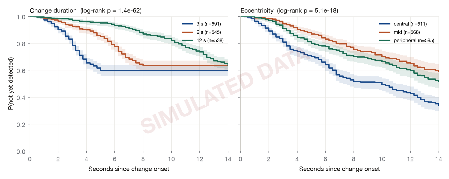
Time from change onset to the response, with non-detections right-censored at the end of the hold window (1041 of 1674 trials, 62%). Discarding those trials would bias every latency estimate toward the easy changes; every model here keeps them.

01 Survival

Kaplan–Meier

Survival curves — **P(not yet detected) since change onset.** *Log-rank by duration p = p = 1.4e-62; by eccentricity p = p = 5.1e-18; by type p = p = 1.7e-10.*

Median time to detection (s) by condition; ∞ when fewer than half were detected
condition	n	detections	median (s)
duration = 3000	591	238	∞
duration = 6000	545	200	∞
duration = 12000	538	195	∞
ecc_bin = central	511	269	9.96
ecc_bin = mid	568	157	∞
ecc_bin = peripheral	595	207	∞
type = appear	238	123	9.05
type = brightness	233	94	12.76
type = disappear	236	105	12.00
type = hue	237	71	∞
type = orientation	241	56	∞
type = position	241	98	12.91
type = size	248	86	∞

02 Cox models

Proportional hazards, fixed and time-varying

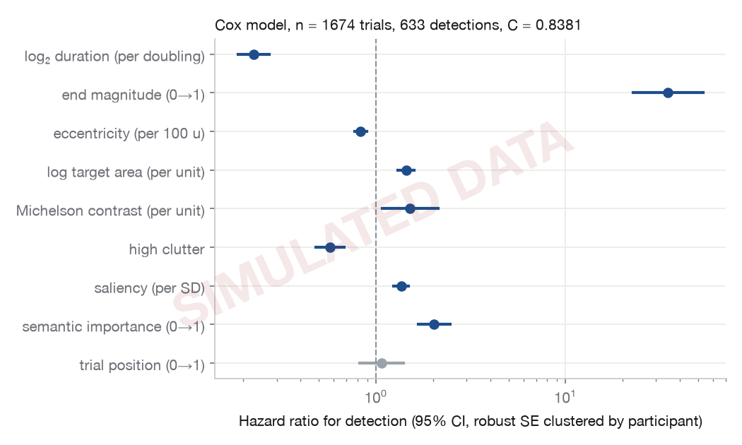
Cox forest plot — **Hazard ratios.** *n = 1674, events = 633, concordance 0.838; robust SE clustered by participant.*

Cox PH with end magnitude as a fixed covariate
term	β	SE	HR	95% CI (β)	p
log2_duration	-1.486	0.096	0.226	[-1.67, -1.30]	p = 4.4e-54
magnitude_norm	3.546	0.216	34.667	[3.12, 3.97]	p = 2.8e-60
ecc_100u	-0.185	0.039	0.831	[-0.26, -0.11]	p = 1.7e-6
log_area_c	0.365	0.052	1.441	[0.26, 0.47]	p = 2.4e-12
contrast_c	0.414	0.173	1.512	[0.07, 0.75]	p = 0.017
clutter_high	-0.557	0.087	0.573	[-0.73, -0.39]	p = 1.3e-10
sal_z	0.306	0.045	1.359	[0.22, 0.39]	p = 1.1e-11
target_importance	0.706	0.099	2.025	[0.51, 0.90]	p = 8.2e-13
trial_frac	0.070	0.136	1.072	[-0.20, 0.34]	p = 0.609
type_appear	0.527	0.138	1.694	[0.26, 0.80]	p = 1.3e-4
type_brightness	0.327	0.159	1.386	[0.01, 0.64]	p = 0.040
type_disappear	0.426	0.149	1.532	[0.13, 0.72]	p = 0.004
type_orientation	-0.378	0.173	0.685	[-0.72, -0.04]	p = 0.029
type_position	0.563	0.168	1.756	[0.23, 0.89]	p = 8.1e-4
type_size	0.370	0.141	1.448	[0.09, 0.65]	p = 0.009

Proportional-hazards test (Schoenfeld residuals, rank transform): violations at p < 0.01 for no term. A violation for end magnitude is expected and informative: the hazard rises as the change accumulates, so end magnitude cannot have a constant effect over time. The time-varying model below addresses this directly.

Cox with time-varying current magnitude (51477 intervals of 0.25 s)
term	β	SE	HR	95% CI (β)	p
magnitude_now	1.718	0.474	5.573	[0.79, 2.65]	p = 2.9e-4
log2_rate	0.980	0.161	2.664	[0.66, 1.29]	p = 1.1e-9
ecc_100u	-0.184	0.034	0.832	[-0.25, -0.12]	p = 6.3e-8
log_area_c	0.365	0.049	1.441	[0.27, 0.46]	p = 1.1e-13
contrast_c	0.395	0.202	1.485	[0.00, 0.79]	p = 0.050
clutter_high	-0.553	0.088	0.575	[-0.73, -0.38]	p = 3.5e-10
sal_z	0.314	0.045	1.369	[0.23, 0.40]	p = 2.2e-12
target_importance	0.706	0.134	2.026	[0.44, 0.97]	p = 1.4e-7
type_appear	0.480	0.152	1.616	[0.18, 0.78]	p = 0.002
type_brightness	0.324	0.160	1.383	[0.01, 0.64]	p = 0.043
type_disappear	0.362	0.157	1.437	[0.06, 0.67]	p = 0.021
type_orientation	-0.375	0.183	0.687	[-0.73, -0.02]	p = 0.041
type_position	0.581	0.166	1.787	[0.26, 0.90]	p = 4.5e-4
type_size	0.355	0.167	1.426	[0.03, 0.68]	p = 0.033

magnitude_now is the normalised magnitude reached by the end of each interval; log2_rate = log2(magnitude_norm / duration_s).

Sensitivity: same model on all main-phase change trials including flagged ones (n = 2116)
term	β	SE	HR	95% CI (β)	p
log2_duration	-1.431	0.086	0.239	[-1.60, -1.26]	p = 2.3e-62
magnitude_norm	3.357	0.188	28.717	[2.99, 3.73]	p = 3.9e-71
ecc_100u	-0.187	0.036	0.829	[-0.26, -0.12]	p = 2.1e-7
log_area_c	0.362	0.047	1.437	[0.27, 0.45]	p = 1.7e-14
contrast_c	0.418	0.155	1.520	[0.11, 0.72]	p = 0.007
clutter_high	-0.530	0.066	0.588	[-0.66, -0.40]	p = 5.9e-16
sal_z	0.251	0.042	1.285	[0.17, 0.33]	p = 2.6e-9
target_importance	0.539	0.107	1.714	[0.33, 0.75]	p = 5.0e-7
trial_frac	0.097	0.133	1.102	[-0.16, 0.36]	p = 0.463
type_appear	0.462	0.126	1.587	[0.22, 0.71]	p = 2.4e-4
type_brightness	0.257	0.140	1.293	[-0.02, 0.53]	p = 0.067
type_disappear	0.409	0.146	1.506	[0.12, 0.70]	p = 0.005
type_orientation	-0.277	0.156	0.758	[-0.58, 0.03]	p = 0.076
type_position	0.560	0.152	1.752	[0.26, 0.86]	p = 2.3e-4
type_size	0.391	0.136	1.478	[0.12, 0.66]	p = 0.004

03 Accelerated failure time

AFT alternatives

AFT models describe covariates as stretching or compressing time-to-detection (time ratio = e^β). Weibull AIC 3960.66 vs log-logistic AIC 4017.06; concordance 0.838 vs 0.839.

Weibull AFT (β > 0 = later detection)
term	β	SE	time ratio	95% CI (β)	p
clutter_high	0.251	0.039	1.285	[0.17, 0.33]	p = 1.2e-10
contrast_c	-0.178	0.087	0.837	[-0.35, -0.01]	p = 0.040
ecc_100u	0.081	0.015	1.084	[0.05, 0.11]	p = 7.6e-8
log2_duration	0.606	0.022	1.833	[0.56, 0.65]	p < 1e-100
log_area_c	-0.161	0.022	0.851	[-0.20, -0.12]	p = 1.4e-13
magnitude_norm	-1.559	0.085	0.210	[-1.73, -1.39]	p = 2.6e-75
sal_z	-0.132	0.020	0.877	[-0.17, -0.09]	p = 2.3e-11
target_importance	-0.319	0.059	0.727	[-0.44, -0.20]	p = 7.1e-8
trial_frac	-0.030	0.061	0.970	[-0.15, 0.09]	p = 0.620
type_appear	-0.232	0.066	0.793	[-0.36, -0.10]	p = 4.6e-4
type_brightness	-0.152	0.070	0.859	[-0.29, -0.01]	p = 0.030
type_disappear	-0.196	0.069	0.822	[-0.33, -0.06]	p = 0.004
type_orientation	0.154	0.080	1.166	[-0.00, 0.31]	p = 0.055
type_position	-0.248	0.072	0.780	[-0.39, -0.11]	p = 6.0e-4
type_size	-0.173	0.073	0.841	[-0.32, -0.03]	p = 0.018
Intercept	2.007	0.116	7.443	[1.78, 2.23]	p = 2.4e-67

Log-logistic AFT
term	β	SE	time ratio	95% CI (β)	p
clutter_high	0.254	0.043	1.290	[0.17, 0.34]	p = 3.9e-9
contrast_c	-0.136	0.099	0.873	[-0.33, 0.06]	p = 0.167
ecc_100u	0.100	0.017	1.105	[0.07, 0.13]	p = 3.0e-9
log2_duration	0.605	0.024	1.830	[0.56, 0.65]	p < 1e-100
log_area_c	-0.176	0.025	0.839	[-0.22, -0.13]	p = 1.1e-12
magnitude_norm	-1.520	0.084	0.219	[-1.68, -1.36]	p = 2.0e-73
sal_z	-0.133	0.022	0.876	[-0.18, -0.09]	p = 2.2e-9
target_importance	-0.302	0.064	0.739	[-0.43, -0.18]	p = 2.5e-6
trial_frac	-0.051	0.068	0.951	[-0.18, 0.08]	p = 0.459
type_appear	-0.236	0.075	0.790	[-0.38, -0.09]	p = 0.002
type_brightness	-0.107	0.078	0.898	[-0.26, 0.05]	p = 0.171
type_disappear	-0.167	0.075	0.847	[-0.31, -0.02]	p = 0.027
type_orientation	0.184	0.086	1.203	[0.02, 0.35]	p = 0.032
type_position	-0.216	0.080	0.806	[-0.37, -0.06]	p = 0.007
type_size	-0.107	0.079	0.898	[-0.26, 0.05]	p = 0.175
Intercept	1.746	0.124	5.731	[1.50, 1.99]	p = 1.0e-44

04 Threshold

Magnitude at detection

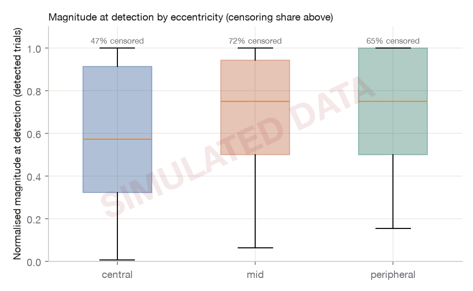
Instead of time, the outcome is the normalised magnitude reached when the participant responded; a missed trial is censored at the end magnitude. Positive coef = larger magnitude needed at detection (threshold up).

Log-normal AFT on the magnitude scale (AIC 1216.39)
term	β	SE	threshold ratio	95% CI (β)	p
clutter_high	0.215	0.045	1.240	[0.13, 0.30]	p = 2.2e-6
contrast_c	-0.050	0.105	0.951	[-0.26, 0.15]	p = 0.630
ecc_100u	0.123	0.018	1.131	[0.09, 0.16]	p = 2.5e-12
log2_duration	-0.014	0.025	0.986	[-0.06, 0.04]	p = 0.570
log_area_c	-0.145	0.026	0.865	[-0.20, -0.09]	p = 2.3e-8
sal_z	-0.145	0.024	0.865	[-0.19, -0.10]	p = 9.1e-10
target_importance	-0.232	0.067	0.793	[-0.36, -0.10]	p = 5.5e-4
type_appear	-0.087	0.078	0.917	[-0.24, 0.07]	p = 0.266
type_brightness	0.008	0.082	1.008	[-0.15, 0.17]	p = 0.926
type_disappear	-0.011	0.079	0.989	[-0.16, 0.14]	p = 0.890
type_orientation	0.158	0.088	1.171	[-0.01, 0.33]	p = 0.072
type_position	-0.134	0.083	0.875	[-0.30, 0.03]	p = 0.105
type_size	0.022	0.083	1.022	[-0.14, 0.18]	p = 0.794
Intercept	-0.333	0.111	0.717	[-0.55, -0.11]	p = 0.003

Magnitude at detection by eccentricity — **Threshold rises with eccentricity.** *Detected trials only in the boxes; censoring share above.*